4 minutes
Tidy Monte Carlo simulations
Simulation studies are extremely useful for understanding how statistical methods work, what happens when you violate their assumptions, for calculating statistical power, for understanding the consequences of p-hacking, and many other things. However, they can also be somewhat inaccessible or have a steep learning curve. In order to make them more accessible for people already familiar with {tidyverse} packages such as {dplyr} and {tidyr} and the concept of Tidy Data, I spent some time constructing a general workflow for simulations within a tidy workflow using {purrr}.
This workflow maximizes transparency of the steps by retaining all generated data sets and results. It also maximises code reusability by separating the key steps of simulating (define experiment conditions, generate data, analyse data, iterate, summarise across iterations) into separate functions and code blocks. This post illustrates a simple example of this workflow to calculate the false positive rate and false negative rate (power) of a Student’s t-test for a given population effect size. Of course, this is easier to calculate in G*power, but it provides a simple example of the workflow, which can be used for much more complex things.
Dependencies
library(tidyr)
library(dplyr)
library(purrr)
library(janitor)
library(ggplot2)
library(scales)
library(knitr)
library(kableExtra)
Define data generation function
Generate two datasets sampled from a normally distributed population, with equal SDs and custom N per group and population means (\(\mu\)).
# functions for simulation
generate_data <- function(n_per_condition,
                          mean_control,
                          mean_intervention,
                          sd) {

  data_control <-
    tibble(condition = "control",
           score = rnorm(n = n_per_condition, mean = mean_control, sd = sd))

  data_intervention <-
    tibble(condition = "intervention",
           score = rnorm(n = n_per_condition, mean = mean_intervention, sd = sd))

  data_combined <- bind_rows(data_control,
                             data_intervention)

  return(data_combined)
}
Define analysis function
Apply an independent Student’s t-test to the data and extract the p-value as a column in a tibble.
analyze <- function(data) {

  res_t_test <- t.test(formula = score ~ condition,
                       data = data,
                       var.equal = TRUE,
                       alternative = "two.sided")

  res <- tibble(p = res_t_test$p.value)

  return(res)
}
Define experiment conditions
Use expand_grid() to create a tibble of all combinations of all each level of each variable, plus an arbitary number of iterations for the simulation.
# simulation parameters
experiment_parameters <- expand_grid(
  n_per_condition = 50,
  mean_control = 0,
  mean_intervention = c(0, 0.5),
  sd = 1,
  iteration = 1:10000
) |>
  # because mean_control is 0 and both SDs are 1, mean_intervention is a proxy for Cohen's d.
  # because d = [mean_intervention - mean_control]/SD_pooled
  # for clarity, let's just make a variable called population_effect_size
  mutate(population_effect_size = paste0("Cohen's d = ", mean_intervention))
Run simulation
Use {purrr}’s parallel map function (pmap()) to map the data generation and analysis functions onto the experiment parameters. This saves the (tidy) output of each function as a nested data column.
# set seed
set.seed(42)

# run simulation
simulation <- experiment_parameters |>
  mutate(generated_data = pmap(list(n_per_condition = n_per_condition,
                                    mean_control = mean_control,
                                    mean_intervention = mean_intervention,
                                    sd = sd),
                               generate_data)) |>
  mutate(results = pmap(list(generated_data),
                        analyze))
Run results across iterations
Unnest the nested data in the results column and then, for each of the experiment conditions, summarize the proportion of significant p-values iterations. Print a plot of the results.
# summarize across iterations
simulation_summary <- simulation |>
  # unnest results
  unnest(results) |>
  # for each level of mean_intervention...
  group_by(population_effect_size) |>
  # ... calculate proportion of iterations where significant results were found
  mutate(significant = p < .05) |>
  summarize(proportion_of_significant_p_values = mean(significant))

# plot results
ggplot(simulation_summary, aes(population_effect_size, proportion_of_significant_p_values)) +
  geom_col() +
  theme_linedraw() +
  scale_y_continuous(breaks = breaks_pretty(n = 10),
                     labels = label_percent(),
                     limits = c(0,1),
                     name = "Proportion of significant p-values") +
  scale_x_discrete(name = "Population effect size")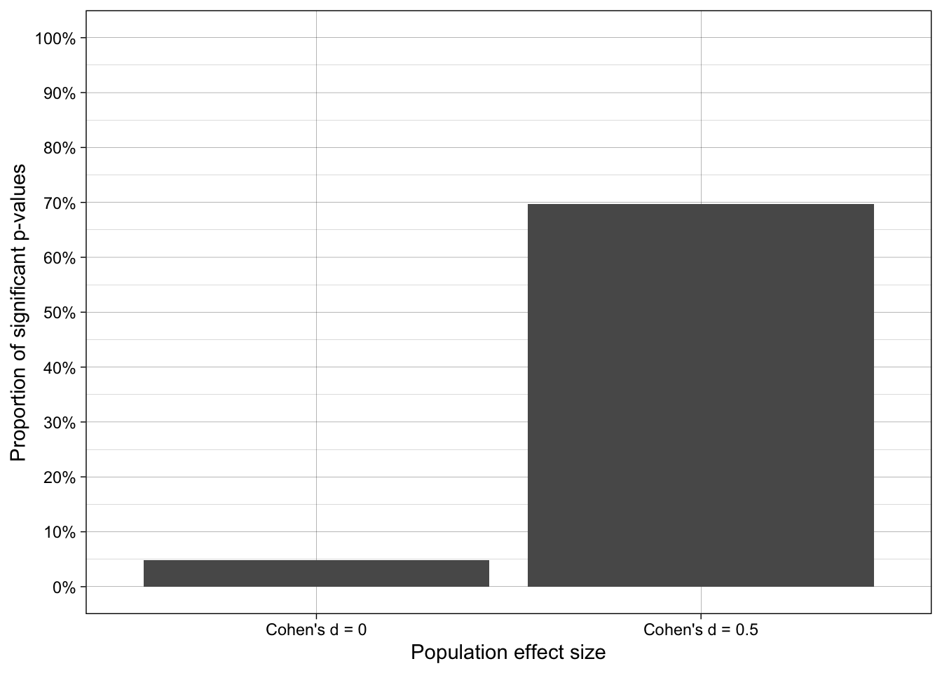
- When population effect size is zero, the false positive rate is 5%, as it should be given that a) all assumptions of the test were met by the data generating process and b) the number of iterations was sufficiently high.
- When population effect size is Cohen’s d = 0.5 and N = 50 per group, statistical power (1-false negative rate) c.70% when all assumptions of the test were met by the data generating process.
Masters course based on this workflow
Building on this general workflow, I teach a Masters-level course “Improving your statistical inferences through simulation studies in R” at the University of Bern in Spring semester. Materials for the course are freely available under an Open Source license (CC-BY 4.0).
Resources
- Pustejovsky & Miratrix, 2023, Designing Monte Carlo Simulations in R. https://jepusto.github.io/Designing-Simulations-in-R/
- Siepe et al. (2024) Simulation Studies for Methodological Research in Psychology: A Standardized Template for Planning, Preregistration, and Reporting. Psychological Methods. https://doi.org/10.1037/met0000695